GFN 2019 – Gateway Matrix

Gateway Matrix Remodeled

Gateway Matrix Remodeled

From so-called experts and politicians we always hear talk about vaping as the possible "Gateway to Smoking". Everybody knows--or at least should know--there is more than one possible gateway. Clive Bates described them in his blog post.  Riccardo Polosa et al. presented A Risk Assessment Matrix for Public Health Principles: The Case for E-Cigarettes. That inspired me to quantify the gateways in a probability matrix.

But first I found that I had to find a metric to evaluate the output of such a matrix. A basically very simple concept came to mind: The Total Harm Risk Metric (THRM) was born.

This is part two of video poster #32 presented at the Global Forum on Nicotine (GFN) 2019.

You find the raw poster (without sound) here: <click>

An edited version with audio comment will soon be published on our youtube channel.

Back to the Gateways ...

The Problem

When survey results are presented, concerned comments about "Vaping as a possible Gateway to Smoking" seem inevitable. But is it really just a one way street as those comments insinuate?

What about other possible Gateways?


Reality is a Matrix

Well, there actually is a Gateway from each behavior to each other. Including itself. What we have here is a square Matrix where none fall out of the system and they all end up in one category or another. How many of the original set stay in the same behavioral group, and how many take the Gateway to another, all depends on the probability of the individual Gateway. Like this:

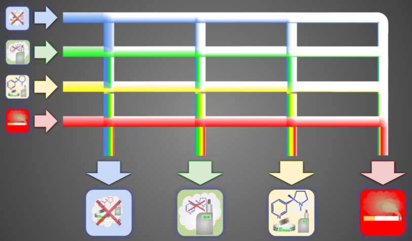
But of course the Matrix is more complex than this, since there are many more distinct categories, like those I identified in THRM.
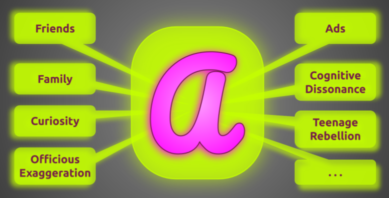
Attractivity

The hard part is to guesstimate reasonable probabilities for each Gateway.

It's even harder, because a useful model also works with environmental variables that have an influence on the results. To keep it simple I only use a single variable with a linear influence on the probabilities. This would be a factor describing an "Attractivity" of smokeless products in general. Many influences are accumulated into it:
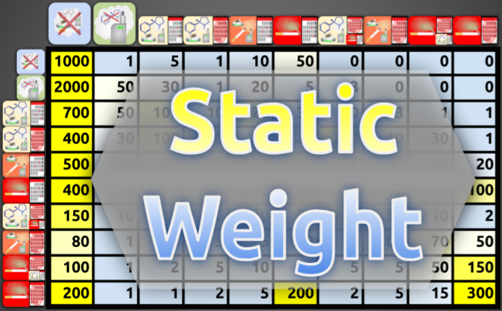
 

Weights

For each row in the Gateway Probability Matrix the total sum must be 1.0. One way to manage this is to use arbitrary weights that are all relative to the other weights in only the same row. In the end all weights are added and the weight for each column is divided by this sum. Resulting in the actual probability.

There are two sets of weights. One is the static weight that is the constant base value.

The other is the dynamic weight. Each number here will be multiplied by the Attractivity before it's added to the static weight value to create the adjusted column weight.

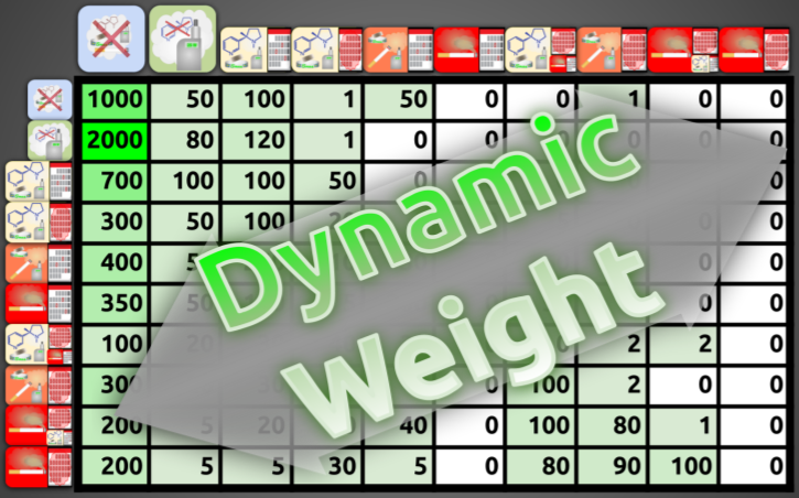
Finding reasonable weights is a bit tricky. I started with what seemed plausible. Then I tweaked the numbers so that the results of the model (see below) roughly fit to the data from the NYTS studies. More time, effort, and some intelligent (genetic?) algorithm could produce a much better fit.


Probabilities

The resulting probability matrix is the core of the modeling. Only one environmental variable has an external influence on the model: the Attractivity.

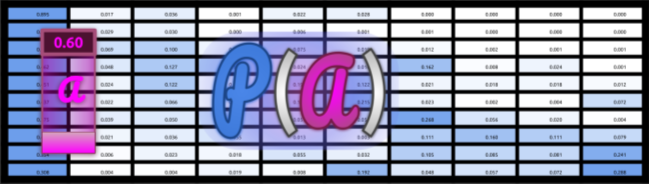
The process itself is very simple:

  1. start with a known vector of data
  2. calculate the probability matrix according to the next selected Attractivity
  3. do a matrix multiplication with the input vector
  4. the resulting vector is also the input for the next iteration (2.)


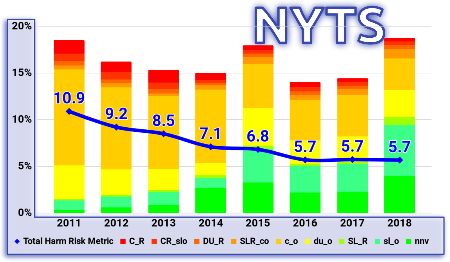
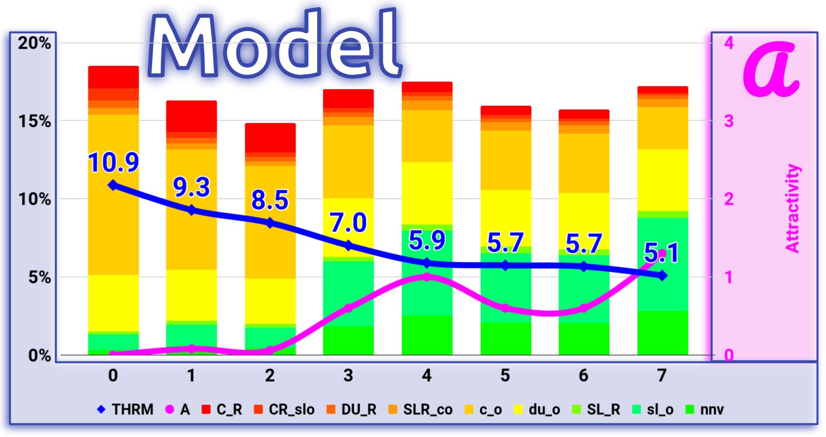
Model compared to NYTS
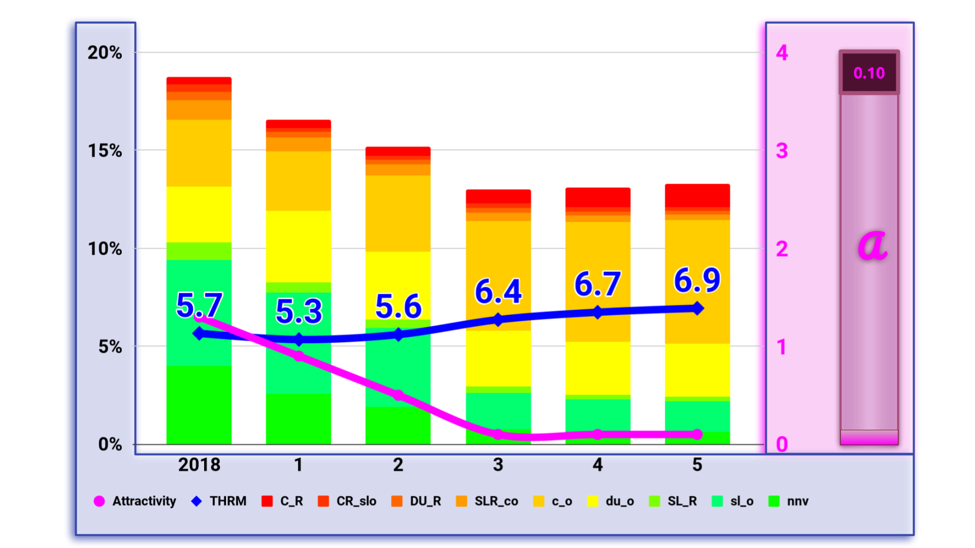
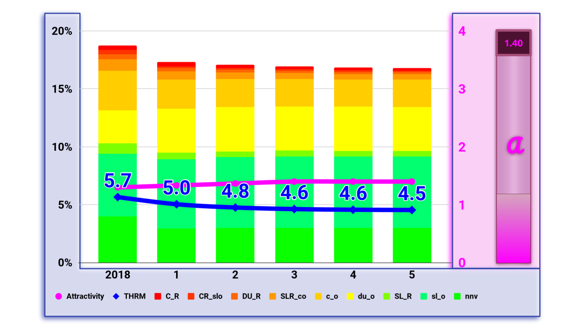
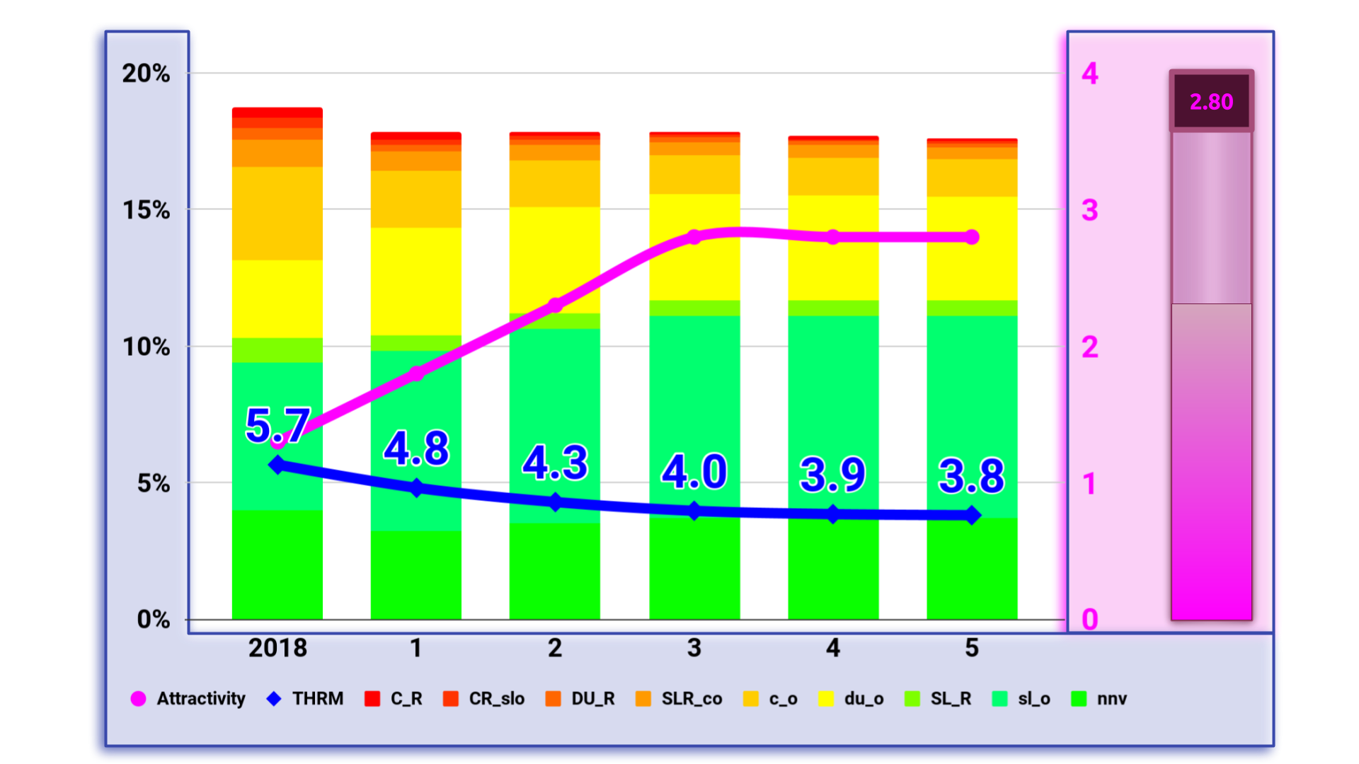
Possible futures

Starting with the NYTS data from 2018 I calculated the model for different scenarios from total reduction of the Attractivity via prohibitive regulations and propaganda to massive support to increase it. Here are some results:
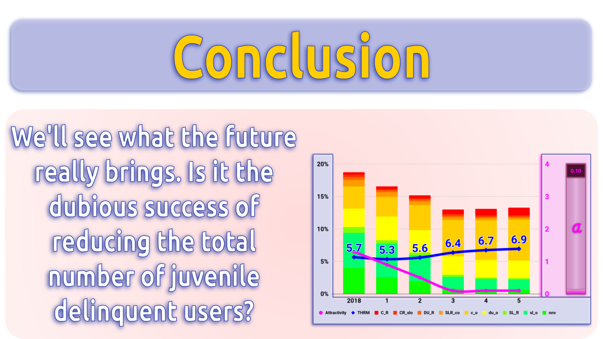
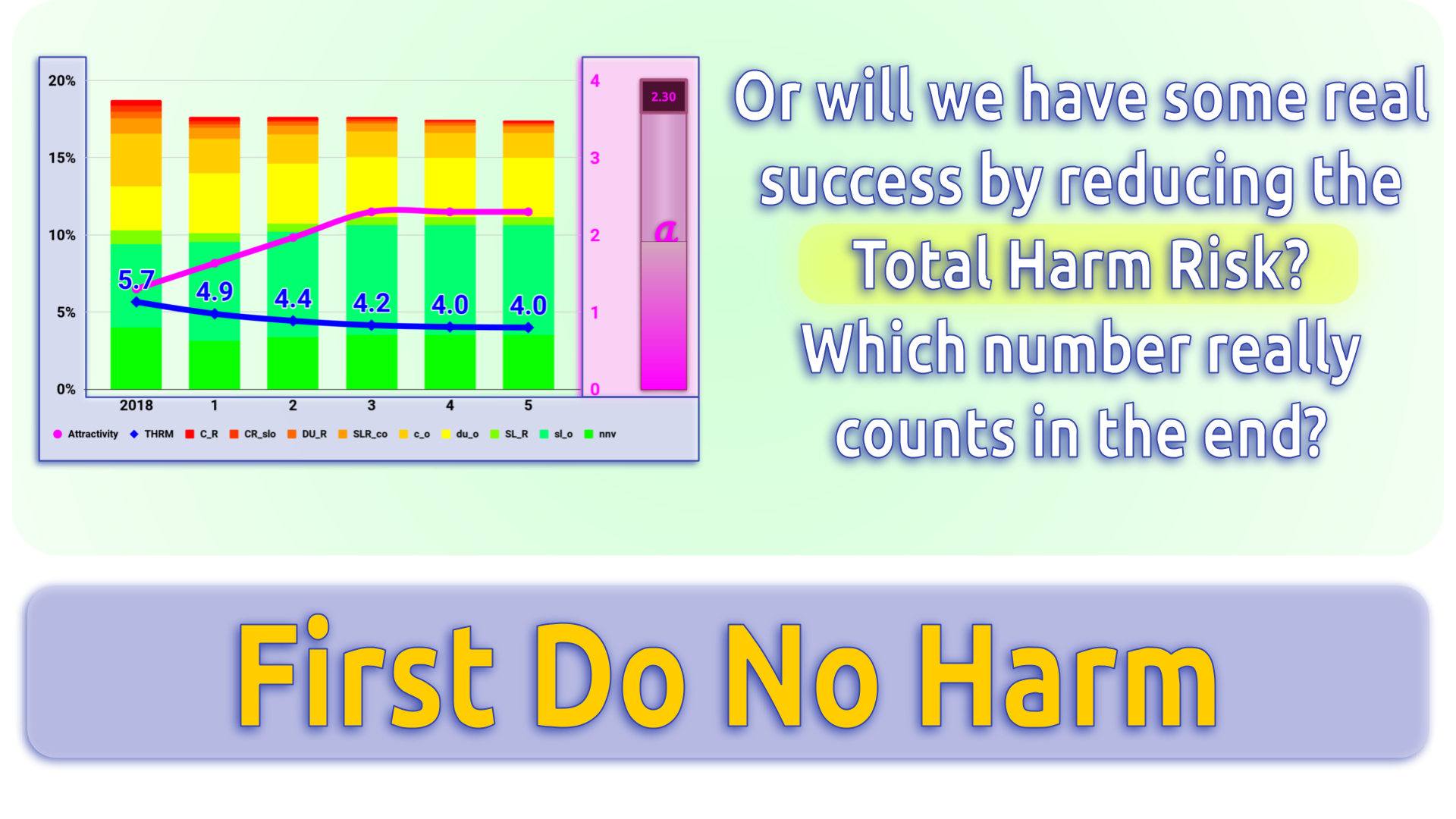
 

Conclusion

Technical Details

Sources and Calculations

I did all the calculations with Google spreadsheets. For the modelling and the animations in the video with a variable Attractivity factor I used the built-in scripting (JavaScript) to calculate the probabilities. The formulas in the script are exactly the same as in the spread sheets and the weight data is taken from there. You can download the sheet, ".xlsx" format works best. Some cosmetic formulas (names) won't work and some graphs become really ugly, but all the important calculations are done correctly.

The spreadsheet Gateway Matrix contains several sheets. Some of them were used to calculate the animations, some are illustrating the influence of the Attractivity factor. The scripts are Gateways.gs, which does the calculation and modeling and export_anims.gs, which I used to export tables and graphics to Google slides.

  • Matrix: the main sheet. It contains several tables and the main inputs. The results here are calculated exclusively with regular spreadsheet formulas. No scripts necessary. Due to this limitation, the tables on this sheet can only calculate the results for a single value of Attractivity (A3), not the dynamic changes required for the real model. Rows:
    • 3: Main inputs. Modifying these values affect everything.
      • A3 - Attractivity factor for the dynamic weight in calculating the probability matrix.
      • C3-L3 - Risk factors for the THRM calculation and the Desirability matrix (5/65).
    • 5: Desirability matrix. Didn't make it into the presentation. This simply calculates the desirability of the Gateway based on the differences in the categorical risk factors.
    • 20: Static Weight matrix. Input for calculating the probability.
    • 35: Dynamic Weight matrix. Input for calculating the probability. Multiplied by the Attractivity factor (A3)
    • 50: Probability matrix. Calculated from Static Weight (20) + Attractivity (A3) * Dynamic Weight (35)
    • 65: Weighted Desirability matrix. (Not used in the presentation.) Numbers from the Desirability matrix (5) multiplied by the Probability (50).
    • 80: Modeling with a static Attractivity (A3).
      • The initial data (81) is a copy of the NYTS 2011 data.
      • Each of the following rows (82-87) is calculated by matrix multiplication of the previous row with the Probability matrix.
    • 108: Accumulation of the resulting iterations for the modeling with different static Attractivities on the sheets AttrXXX.
  • Model: calculated with the script
  • Predict: Used by the script to calculate the predictions animation for a range of final Attractivity values. As start data I used the numbers from the NYTS 2018.
  • Attr_gen: Used by the script to generate the probability matrix tables for the animation.
  • AttrXXX: Modeling for different static values of Attractivity. The results (row 33) are used on the main sheet (Matrix:108).

Methods

As already mentioned, the modeling process itself is pretty simple. A matrix multiplication of the previous data row with the probability matrix calculated with the guesstimated Attractivity factor for this row. The hard part is getting the Probability matrix right. This is an iterative process. I started with weights that seemed reasonable. Of course, the resulting data started soon to deviate from the original data. So I looked at where the deviations were strongest and adjusted the weights. Several times until the model was a reasonably good match for the existing data.

Now that the model is tested against existing data, I can use it to predict the near future with different scenarios for the Attractivity factor.

Improving

Algorithm

Manually adjusting the weights isn't very practical and it takes quite some time to get a satisfying fit. It can be automated. I would suggest programming a genetic algorithm to do the job. Each row of weights (static & dynamic) is a "gene". As a measure for the "fit" we can use the accumulated errors (deviations) in each category of each year. As input for the algorithm we also need the summed deviations per column. The genetic algorithm works this way:

  • Mutation: Introduce random variations in the genome. Only a few weights per gene (row) at a time. Too many changes at once would hinder the optimization. Pure random would also be too erratic, so the range of the variations should be limited by the original value and the total deviation in the column.
  • Selection: After generating a zoo (maybe 100) of mutated models, we automatically select the 3-5 best fits (lowest total deviation).
  • Breeding: Generating children (again maybe 100) by randomly selecting a gene (row) from one of the remaining champions.
  • Selection: The best fitting 3-5 children (or parents) are chosen for the next iteration.
  • Evaluation: If the original model is still the best fit, we stop, as that is probably as good as it gets.
  • Repeat: As long as there are improvements, we start again with mutations. Now with several initial models to mutate. Using not the single best fit helps avoiding getting stuck at a local optimum instead of reaching a global optimum.

Now we use the best fitting model to similarly adjust the Attractivity factor to get even better fits.

Granularity

We usually only have annual data to test the model against. But in real life most people tend to stay in transitory categories a much shorter time. Also the Attractivity tends to have short term spikes caused by viral media hypes and ad campaigns. Thus it would be closer to reality to create the model to produce several (e.g. monthly) intermediate results.

More Variables

I used a single abstract value "Attractivity" as an input variable. It's rather easy to introduce more external variables. Just add another table of dynamic weights for each variable. But make sure that these variables are as independent as possible. More than 2 or 3 variables might be too much for the genetic algorithm to handle at once. It's also hard to make comprehensible predictions when more variables are involved.

Conclusion

The model is pretty simple, but can be adapted to model reality as presented in data. The beauty of this model is that it only relies on actual  statistical data. No need for speculations on individual behavioral changes, except for the initial setup of the weight tables. But that speculation bias is eliminated by the fitting of the model. The more statistical data as input the more reliable the model gets to predict the near future.


4 Gedanken zu „GFN 2019 – Gateway Matrix

  1. Da wäre eine deutsche Übersetzug sicher spannend.
    Ihr wollt doch deutsche Dampfer erreichen oder nicht ?

  2. Hallo Thomas, danke für den Hinweis, und wir arbeiten bereits dran. Wird trotzdem noch ein kleines Weilchen dauern.

    LG, Hazel

Schreibe einen Kommentar

Deine E-Mail-Adresse wird nicht veröffentlicht. Erforderliche Felder sind mit * markiert